Question 4
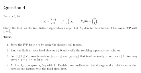
For , let Study the limit as the two distinct eigenvalues merge. Let denote the solution of the same IVP with .
Tasks
Solve the IVP for by using the distinct real modes.
Find the limit at each fixed time as and verify the resulting repeated-root solution.
For , prove bounds on and that tend uniformly to zero as . You may use for .
At , compare with . Explain how coefficients that diverge and a relative error that persists can coexist with the fixed-time limit.
Show solutionHide solution
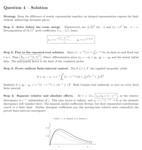
Question 4 – Solution
Strategy. Keep the difference of nearby exponentials together; an integral representation exposes the limit without subtracting divergent pieces.
Step 1: Solve before the roots merge. Eigenvectors are for and for . Decomposition of gives coefficients , hence
Step 2: Pass to the repeated-root solution. Since , its limit at each fixed real is . Thus . Direct differentiation gives , and the stated initial data. The polynomial factor is the limit of the combined modes.
Step 3: Prove uniform finite-interval control. For , the supplied inequality yields Similarly . Both bounds tend uniformly to zero on every fixed finite interval.
Step 4: Separate relative and absolute effects. At , , so the relative discrepancy is , independent of . This time moves to infinity, and , so the absolute discrepancy still vanishes there. The separate modal coefficients diverge, but their exponential contributions cancel to a finite limit. Neither divergent coefficients nor this moving-time relative error contradicts the proved finite-interval convergence.
See the diagram in the original worksheet below.