Solutions to Systems — Question 7

Question 7 – Solution

Strategy. Derive explicit solutions, then distinguish the algebraic formula’s domain from the connected interval of an initial-value solution.

Step 1: Solve and verify, retaining the zero case. For $a\ne 0$, separation gives $1/x=1/a-t$, hence $$\boxed{X_a(t)=\left(\frac{a}{1-at},e^{-t}\right)^T.}$$ The first derivative is $a^2/(1-at)^2=x^2$, and the data match at $0$. For $a=0$, the solution is $\boxed{X_0=(0,e^{-t})^T}$; local uniqueness of the smooth field excludes other departures from $x=0$.

Step 2: Find the maximal connected intervals. The first component blows up at $1/a$ when $a\ne 0$. Thus $$\boxed{a>0:\ (-\infty,1/a);\qquad a=0:\ \mathbb R; \qquad a<0:\ (1/a,\infty).}$$ The exponential component introduces no further restriction. A finite-valued continuous extension across the pole is impossible. Smoothness is a local regularity condition and does not prevent unbounded growth in finite time.

Step 3: Reject a disconnected continuation. At $a=1$, the formula gives $x(2)=-1$, but the IVP through $0$ exists only for $t<1$. Its first component tends to $+\infty$ as $t\uparrow 1$. The branch for $t>1$ solves the differential equation separately; it cannot be joined into a classical solution through the intervening pole.

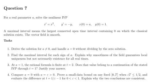
Step 4: Compare finite-time and long-time sensitivity. For $0\le t\le T$ with $\varepsilon T\le 1/2$, $$\|X_\varepsilon(t)-X_0(t)\|=\frac{\varepsilon}{1-\varepsilon t} \le 2\varepsilon.$$ But at $t=1/\varepsilon-1$, still before the pole, the difference equals $1$. That comparison time tends to infinity as $\varepsilon\downarrow 0$. There is no contradiction: closeness on each fixed finite interval does not give a uniform bound over arbitrarily long, parameter-dependent times. The plot shows only the initial-value branches before their poles.