Boundary Value Problems — Question 1

Question 1 – Solution

Strategy. Solve the initial-value family first, then use the endpoint equation to select its slope.

Step 1: Select the shooting slope. Integrating twice gives $y_s=1+sx-x^3$. The right endpoint is $y_s(1)=s$, so $s=2$ is the unique successful slope. An initial-value problem fixes $s$ directly; the boundary-value problem determines it from a condition at another point.

Step 2: Verify the solution and its extrema. The solution $\boxed{y=1+2x-x^3}$ has $y''=-6x$, $y(0)=1$, $y(1)=2$. Since $y'=2-3x^2$, its maximum occurs at $r=\sqrt{2/3}$: $$\boxed{y_{\max}=1+\frac 43\sqrt{\frac 23}>2,\qquad y_{\min}=y(0)=1.}$$ Thus the endpoint values do not bound this forced response from above.

Step 3: Allow arbitrary endpoint values. Direct integration gives $$\boxed{y_{\alpha,\beta}(x)=\alpha+(\beta-\alpha+1)x-x^3.}$$ This works for every $\alpha,\beta$. The difference of two solutions with the same data satisfies $w''=0$, $w(0)=w(1)=0$, so it is zero, proving uniqueness.

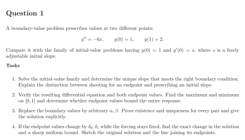
Step 4: Quantify boundary-data sensitivity. The exact response change is $\Delta y=(1-x)\delta_0+x\delta_1$. Therefore $$\boxed{\max_{0\leq x\leq 1}|\Delta y|=\max(|\delta_0|,|\delta_1|).}$$ The inequality follows from convex weights; equality holds at an endpoint. The original curve exceeds its endpoint line $1+x$ by $x-x^3>0$ inside $(0,1)$.