Question 8
An ideal temperature controller is modeled in dimensionless variables. The room temperature is , the target is , and the scaled heater output is . The plant obeys . A controller with memory sets There is no heater saturation, delay or heat-source noise in this ideal model.
Tasks
Convert the plant and controller into a two-state autonomous IVP. Find its equilibrium and explain why is a state rather than a fixed parameter.
Shift to the equilibrium and show it attracts every initial state for every . Classify the eigenvalues at the critical gain.
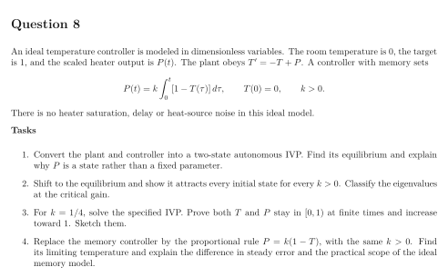
For , solve the specified IVP. Prove both and stay in at finite times and increase toward . Sketch them.
Replace the memory controller by the proportional rule , with the same . Find its limiting temperature and explain the difference in steady error and the practical scope of the ideal memory model.
Show solutionHide solution
Question 8 – Solution
Strategy. The accumulated error supplies an additional state; its equilibrium condition eliminates the temperature offset of proportional feedback.
Step 1: Introduce the controller state. Differentiation gives At equilibrium, and . Heater output depends on accumulated past error, so two states with the same temperature can have different future motion if their current values differ.
Step 2: Check stability and the critical gain. For , , the matrix is . Its roots are . For both are real and negative; at there is a repeated root ; for they are complex with real part . Every homogeneous mode decays, including the polynomial times exponential at the repeated root. Thus the equilibrium attracts every initial state within this ideal linear model.
Step 3: Solve the critical-gain response. Eliminating gives , with . The repeated-root solution and yield The initial values vanish and , . The latter equals , checking the controller equation. The positive subtracted terms and monotonicity imply at finite , and both tend to . Here the heater output stays nonnegative without needing a saturation rule.
Step 4: Compare steady errors. Proportional feedback instead gives , so and the steady error is . The memory controller can retain even when the current error is zero; a proportional controller would then set . Real actuator limits and delays can change stability or feasibility, so the ideal conclusions apply under the stated assumptions, not to every physical controller.
See the diagram in the original worksheet below.