Question 7
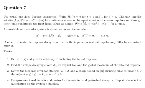
Use causal one-sided Laplace transforms. Write for and for . The unit impulse satisfies for continuous near . Interpret equations between impulses and through their jump conditions; use right-hand values at jumps. Write for a jump.
An unstable second-order system is given one corrective impulse: Choose to make the response decay to zero after the impulse. A realized impulse may differ by a constant error .
Tasks
Derive and for arbitrary , including the initial response.
Find the unique decaying choice , its explicit tail and the global maximum of the selected response.
Derive the response error for strength and a sharp bound on ensuring error at most throughout , where .
Compare exact real transform domains for the selected and perturbed strengths. Explain the effect of cancellation on the system’s stability.
Show solutionHide solution
Question 7 – Solution
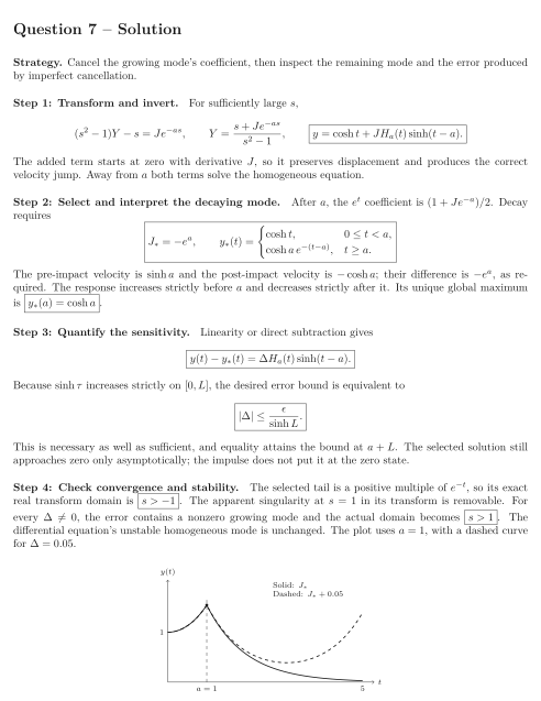
Strategy. Cancel the growing mode’s coefficient, then inspect the remaining mode and the error produced by imperfect cancellation.
Step 1: Transform and invert. For sufficiently large , The added term starts at zero with derivative , so it preserves displacement and produces the correct velocity jump. Away from both terms solve the homogeneous equation.
Step 2: Select and interpret the decaying mode. After , the coefficient is . Decay requires The pre-impact velocity is and the post-impact velocity is ; their difference is , as required. The response increases strictly before and decreases strictly after it. Its unique global maximum is .
Step 3: Quantify the sensitivity. Linearity or direct subtraction gives Because increases strictly on , the desired error bound is equivalent to This is necessary as well as sufficient, and equality attains the bound at . The selected solution still approaches zero only asymptotically; the impulse does not put it at the zero state.
Step 4: Check convergence and stability. The selected tail is a positive multiple of , so its exact real transform domain is . The apparent singularity at in its transform is removable. For every , the error contains a nonzero growing mode and the actual domain becomes . The differential equation’s unstable homogeneous mode is unchanged. The plot uses , with a dashed curve for .
See the diagram in the original worksheet below.