Nonconstant Coefficient IVP’s — Question 4

Question 4 – Solution

Strategy. A vanishing leading coefficient imposes compatibility. Boundedness at the singular endpoint can replace a free constant that would exist away from it.

Step 1: Inspect the singular endpoint. At zero, the equation requires $2y(0)=1$, so the given datum is compatible. For $t>0$, multiplying by $t$ gives $(t^2y)'=te^{-t}$. Its general integral has an additive constant in $t^2y$. Boundedness of $y$ forces that constant to be zero, hence $$\boxed{y(t)=\frac{1-(1+t)e^{-t}}{t^2}\quad(t>0).}$$ This proves uniqueness among bounded solutions near zero, without invoking a regular-IVP theorem at a singular point.

Step 2: Solve in transform space. The full rule $\mathcal L\{ty'\}=-Y-sY'$ gives $Y-sY'=1/(s+1)$. Therefore $$(Y/s)'=-\frac 1{s^2(s+1)},\qquad Y=s\int_s^\infty\frac{du}{u^2(u+1)} =\boxed{1-s\ln\frac{s+1}{s}},\quad s>0.$$ The omitted homogeneous term is $Cs$ and cannot tend to zero. The inverse below verifies boundedness and transform existence.

Step 3: Verify the endpoint and forward transform. A nonsingular representation is $y(t)=\int_0^1 u e^{-ut}\,du$, including at zero. Thus $y(0)=1/2$, $y'(0)=-1/3$, and differentiation verifies the original equation (or use $(t^2y)'=te^{-t}$ for $t>0$ and compatibility at zero). For $s>0$, integrating first in time gives $$Y(s)=\int_0^1\frac{u}{s+u}\,du=1-s\ln\frac{s+1}{s}.$$ The finite absolute double integral justifies interchange.

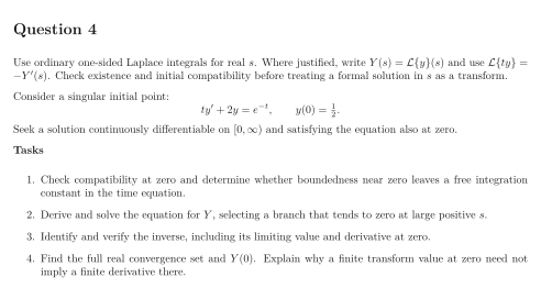
Step 4: Check the boundary rather than just the formula. The function is positive and $y(t)\sim 1/t^2$. Therefore the exact real convergence set is $\boxed{[0,\infty)}$, with divergence for negative $s$. At zero the same nonnegative double integral gives $\boxed{Y(0)=\int_0^1 1\,du=1}$. But $ty(t)\sim 1/t$, so its first moment diverges. Indeed $Y'(s)=-\ln[(s+1)/s]+1/(s+1)\to-\infty$ as $s\downarrow 0$. A finite boundary area does not imply a finite boundary moment.