Nonconstant Coefficient IVP’s — Question 2

Question 2 – Solution

Strategy. The variable damping gives a growing homogeneous solution in transform space; a genuine transform selects the complementary integral tail.

Step 1: Transform and apply the integrating factor. The equation becomes $sY-1-2Y'=0$, or $$Y'-\tfrac s2Y=-\tfrac 12,\qquad (e^{-s^2/4}Y)'=-\tfrac 12e^{-s^2/4}.$$

Step 2: Impose the transform condition at infinity. For a bounded candidate, $Y=O(1/s)$, so $e^{-s^2/4}Y\to 0$. Integrating to infinity yields $$\boxed{Y(s)=\tfrac 12e^{s^2/4}\int_s^\infty e^{-u^2/4}\,du =e^{s^2/4}\int_{s/2}^\infty e^{-v^2}\,dv.}$$ Any additional $Ce^{s^2/4}$ violates the bound. The recovered inverse will verify boundedness and the entire transform calculation.

Step 3: Identify the inverse and its full domain. Separation in time gives $\boxed{y=e^{-t^2}}$, with $y'=-2te^{-t^2}$ and $y(0)=1$. Completing the square directly gives $$\int_0^\infty e^{-st-t^2}\,dt =e^{s^2/4}\int_{s/2}^\infty e^{-v^2}\,dv.$$ The Gaussian tail is integrable for every real $s$, so this is the exact real domain. This direct verification also justifies the selected transformed branch. Uniqueness follows from the regular first-order equation.

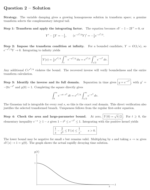
Step 4: Check the area and large-parameter bound. At zero, $\boxed{Y(0)=\sqrt\pi/2}$. For $t\ge 0$, the elementary inequality $e^{-x}\ge 1-x$ gives $1-t^2\le e^{-t^2}\le 1$. Integrating with the positive kernel yields $$\boxed{\frac 1s-\frac 2{s^3}\le Y(s)\le\frac 1s,\qquad s>0.}$$ The lower bound may be negative for small $s$ but remains valid. Multiplying by $s$ and taking $s\to\infty$ gives $sY(s)\to 1=y(0)$. The graph shows the actual rapidly decaying time solution.