Solving IVP’s with Laplace Transforms — Question 8

Question 8 – Solution

Strategy. Transform the accumulated state as well as the instantaneous state. Verify the original integral equation after any differentiation.

Step 1: Transform and complete the square. For sufficiently large $s$, the initial value gives $$sY+Y+Y/s=1/s,\qquad Y=\frac 1{s^2+s+1}.$$ Let $b=\sqrt 3/2$. Completing the square gives $$\boxed{y(t)=\frac 2{\sqrt 3}e^{-t/2}\sin(bt).}$$ This inverts $Y=1/[(s+1/2)^2+b^2]$ with the required sine normalization.

Step 2: Reconstruct the integral and verify. Integration, or differentiation of the following expression, gives $$\boxed{I(t)=1-e^{-t/2}[\cos(bt)+\tfrac 1{\sqrt 3}\sin(bt)].}$$ It satisfies $I(0)=0$ and $I'=y$. Also $y'=e^{-t/2}[\cos(bt)-\sin(bt)/\sqrt 3]$. Substitution yields $y'+y+I=1$ identically, and $y(0)=0$. This checks the undifferentiated problem.

Step 3: Retain the compatibility condition. Differentiation gives $y''+y'+y=0$. Evaluating the original equation at zero gives $\boxed{y'(0)=1}$. Thus the equivalent second-order IVP has data $y(0)=0,y'(0)=1$. If only $y(0)=0$ is retained, a free initial slope remains; it sets the constant value of $y'+y+I$, which need not be one. Conversely, a solution of the differentiated equation with both correct data makes that quantity constant and equal to one, proving equivalence and uniqueness.

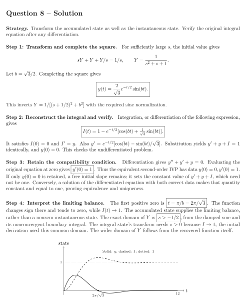
Step 4: Interpret the limiting balance. The first positive zero is $\boxed{t=\pi/b=2\pi/\sqrt 3}$. The function changes sign there and tends to zero, while $I(t)\to 1$. The accumulated state supplies the limiting balance, rather than a nonzero instantaneous state. The exact domain of $Y$ is $\boxed{s>-1/2}$, from the damped sine and its nonconvergent boundary integral. The integral state’s transform needs $s>0$ because $I\to 1$; the initial derivation used this common domain. The wider domain of $Y$ follows from the recovered function itself.