Inverse Laplace Transforms — Question 6

Question 6 – Solution

Strategy. Combine the two large opposite coefficients before taking the coincident-pole limit. An integral representation controls the difference uniformly.

Step 1: Invert before and at collision. For $a\ne 1$, partial fractions give $$F_a=\frac 1{a-1}(\frac 1{s+1}-\frac 1{s+a}),\qquad \boxed{f_a(t)=\frac{e^{-t}-e^{-at}}{a-1}.}$$ At $a=1$, $F_1=(s+1)^{-2}$, so $\boxed{f_1(t)=te^{-t}}$. Both forward transforms verify the original expression. The two individual partial-fraction coefficients diverge as $a\to 1$; their combined inverse has a finite limit.

Step 2: Check sign and the slowest tail. For $a>1$, numerator and denominator of $f_a$ are positive when $t>0$; for $0<a<1$, both are negative. Also $te^{-t}>0$. For unequal poles the slower exponential has a positive, nonzero coefficient, while the other term decays faster. Thus its tail is bounded below by a positive multiple of $e^{-\min(1,a)t}$. Together with direct absolute convergence, this proves the exact domain $$\boxed{s>-\min(1,a).}$$ At $a=1$, the same statement follows from the positive polynomial-exponential tail.

Step 3: Remove the cancellation analytically. Integrating $e^{-(a-1)tv}$ in $v$ gives $$te^{-t}\int_0^1 e^{-(a-1)tv}\,dv =\frac{e^{-t}-e^{-at}}{a-1}$$ when $a\ne 1$ and $t>0$. At $t=0$ both sides extend to zero; at $a=1$ the integral is one, yielding $te^{-t}$. This representation avoids subtracting nearly equal exponentials.

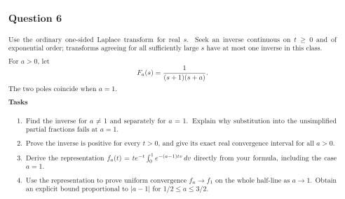
Step 4: Prove uniform half-line convergence. The mean value theorem gives $|e^{-x}-1|\le |x|e^{\max(0,-x)}$. With $m=\min(1,a)$, the representation yields $$|f_a(t)-te^{-t}|\le\frac{|a-1|}{2}t^2e^{-mt}.$$ The maximum of $t^2e^{-mt}$ on $t\ge 0$ occurs at $t=2/m$ and equals $4/(m^2e^2)$. Therefore, for $1/2\le a\le 3/2$, $$\boxed{\sup_{t\ge 0}|f_a(t)-f_1(t)|\le\frac 8{e^2}|a-1|\longrightarrow 0.}$$ This is uniform on the entire half-line, stronger than checking each fixed time. The plotted nearby curves meet at the same zero initial value.