Variation of Parameters — Question 3

Question 3 – Solution

Strategy. The repeated homogeneous root is handled by the Wronskian; an exponential substitution provides an independent residual check.

Step 1: Compute and integrate. The Wronskian is $e^t(1+t)e^t-te^{2t}=e^{2t}$. Hence $$u_1'=-\frac{t}{1+t^2},\qquad u_2'=\frac{1}{1+t^2}.$$ Integrating from zero gives $u_1=-\tfrac 12\ln(1+t^2)$ and $u_2=\arctan t$. Therefore $$\boxed{y=e^t[t\arctan t-\tfrac 12\ln(1+t^2)].}$$ Zero integration endpoints ensure $y(0)=y'(0)=0$.

Step 2: Check by a different calculation. Writing $y=e^tF$ gives $y''-2y'+y=e^tF''$. For the displayed bracket, $$F'=\arctan t,\qquad F''=\frac{1}{1+t^2},\qquad F(0)=F'(0)=0.$$ These identities verify the equation and both data independently. All coefficients and the forcing are continuous on $\mathbb R$, so this is the unique global IVP solution.

Step 3: Prove the sign. For $t>0$, $F(t)=\int_0^t\arctan s\,ds>0$. Equivalently, $F(t)=\int_0^t(t-s)/(1+s^2)\,ds$ has a positive integrand in the interior. Since $e^t>0$, the response is strictly positive.

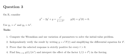
Step 4: Compare the growth rate. For $t>0$, $$\frac{y}{te^t}=\arctan t-\frac{\ln(1+t^2)}{2t}\longrightarrow\boxed{\pi/2}.$$ Although the forcing is smaller than $e^t$ by a factor tending to zero, the zero-data response is asymptotic to $(\pi/2)te^t$. The graph shows the transformed response $F=e^{-t}y$, whose slope tends to $\pi/2$; it is not a plot of $y$ itself.