Question 3
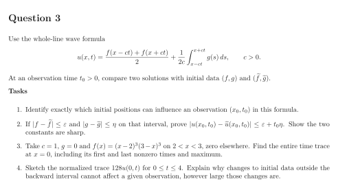
Use the whole-line wave formula At an observation time , compare two solutions with initial data and .
Tasks
Identify exactly which initial positions can influence an observation in this formula.
If and on that interval, prove . Show the two constants are sharp.
Take , and on , zero elsewhere. Find the entire time trace at , including its first and last nonzero times and maximum.
Sketch the normalized trace for . Explain why changes to initial data outside the backward interval cannot affect a given observation, however large those changes are.
Show solutionHide solution
Question 3 – Solution
Strategy. Read causality directly from the interval sampled by the solution formula.
Step 1: Identify the backward interval. Only the initial positions in enter: is sampled at its two endpoints, while is integrated across it. This interval is a sufficient domain of dependence for both types of data; interior values of alone do not enter this one-dimensional formula.
Step 2: Bound and attain the data error. The endpoint contribution is at most . The integral contribution is at most . Hence Constant differences and attain equality. Taking either difference zero proves the corresponding coefficient cannot be improved.
Step 3: Compute the sensor trace. At , . For , the first term is always zero. Thus The trace starts to become nonzero immediately after and returns to zero at . Since , its unique maximum is at . The initial profile is even at its support edges.
Step 4: Interpret finite propagation. At times before , the backward interval does not reach the initial pulse, so the sensor cannot respond. No alteration outside the sampled interval changes either endpoint value or the integral in the formula. This conclusion places no bound on the magnitude of the remote alteration. It is a statement about finite propagation and dependence on initial data, not about small remote effects that have merely been neglected.
See the diagram in the original worksheet below.
