Real Eigenvalues — Question 10

Question 10 – Solution

Strategy. Geometry determines a ratio of modal rates; one elapsed-time observation fixes their common scale.

Step 1: Extract a rate ratio. Initially $u=v=1$, so $u=e^{\lambda t}$ and $v=e^{\mu t}$. The identity $v=u^2$ for every time implies $\mu=2\lambda$. Any $\lambda<0$ with this ratio gives the same oriented orbit as $t$ ranges over the real line. Thus the curve and its arrows alone leave one positive speed factor undetermined.

Step 2: Calibrate the clock. The measurement yields $e^{\lambda\ln 2}=1/2$, so $\lambda=-1$ and $\mu=-2$. Using the specified eigenbasis reconstructs $$\boxed{A=\frac 12\begin{pmatrix}-3&1\\1&-3\end{pmatrix}.}$$

Step 3: Verify the reconstructed trajectory. The solution is $$\boxed{x=e^{-t}+e^{-2t},\qquad y=e^{-t}-e^{-2t}.}$$ Differentiating and multiplying by the displayed matrix agree component by component, and the initial state is $(2,0)^T$. Moreover $u=e^{-t}>0$, $v=e^{-2t}=u^2$, and $u(\ln 2)=1/2$. Every $u>0$ occurs at a finite real time; the limiting origin is excluded from the orbit.

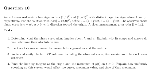
Step 4: Separate geometric and temporal conclusions. As $t\to\infty$, $dy/dx=(1-2e^{-t})/(1+2e^{-t})\to 1$, giving the tangent line $y=x$. On $t\ge 0$, $y'=e^{-t}(2e^{-t}-1)$ changes from positive to negative at $t=\ln 2$. Hence $\boxed{y_{\max}=1/4}$, attained at $x=3/4$. Replacing $A$ by $kA$, $k>0$, changes the solution to $X(kt)$: the oriented curve and maximum value remain the same, but the maximum occurs at $(\ln 2)/k$. Except for $k=1$, it fails the given clock measurement.