Question 3
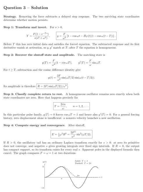
Let for and for . Use one-sided Laplace transforms. Solutions are continuous (and have continuous first derivative for second-order equations); satisfy the equation away from switches and use one-sided derivatives there. Isolated input values do not change the solution.
An undamped oscillator receives a rectangular force of selectable duration: Use the energy .
Tasks
Derive and the delayed step-response formula for .
Find the displacement and velocity at shutoff, and the residual oscillation amplitude.
Classify every duration for which the system remains at rest after shutoff; explain why alone is generally insufficient.
Compute the residual energy and classify the exact real transform domain, including the rest-producing durations.
Show solutionHide solution
Question 3 – Solution
Strategy. Removing the force subtracts a delayed step response. The two surviving state coordinates determine whether motion persists.
Step 1: Transform and invert. For , Before this has zero initial data and satisfies the forced equation. The subtracted response and its first derivative vanish at activation, so match at ; after the equation is homogeneous.
Step 2: Recover the shutoff state and amplitude. The matching state is For , subtraction and the cosine difference identity give Its amplitude is therefore .
Step 3: Classify complete return to rest. A homogeneous oscillator remains zero exactly when both state coordinates are zero. Here that happens precisely for In this particular pulse family, forces and hence also . For a general forcing history, zero displacement alone is insufficient: a nonzero velocity launches a new oscillation.
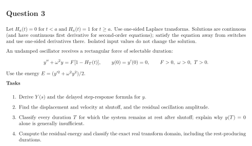
Step 4: Compute energy and convergence. After shutoff, If , the oscillatory tail has an ordinary Laplace transform exactly for : at zero its primitive does not converge, and negative gives growing integrals over fixed sign intervals. If , the output has compact support, so its transform exists for every real . Apparent poles in the displayed formula then cancel. The graph compares at two durations.
See the diagram in the original worksheet below.