Question 6
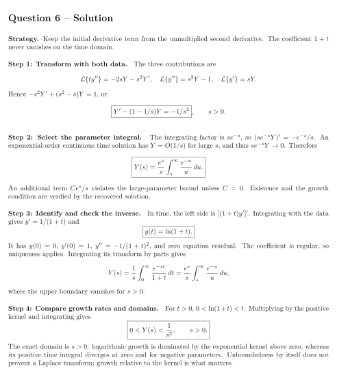
Use ordinary one-sided Laplace integrals for real . Where justified, write and use . Check existence and initial compatibility before treating a formal solution in as a transform.
Solve the regular second-order IVP A convergent parameter integral may be retained in the formula for .
Tasks
Derive the differential equation for , including all initial contributions.
Solve it with an integrating factor and explain the condition that removes its homogeneous term.
Identify and verify the time solution, then check the parameter-integral transform directly.
Prove for and determine the exact real convergence interval. Explain why a growing time solution can still be transformable.
Show solutionHide solution
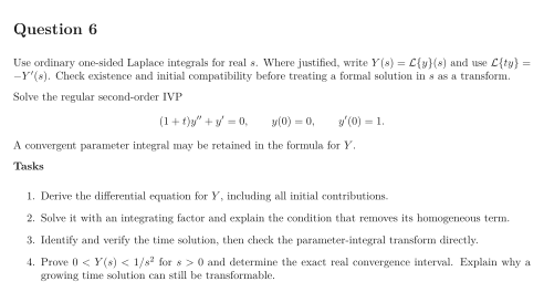
Question 6 – Solution
Strategy. Keep the initial derivative term from the unmultiplied second derivative. The coefficient never vanishes on the time domain.
Step 1: Transform with both data. The three contributions are Hence , or
Step 2: Select the parameter integral. The integrating factor is , so . An exponential-order continuous time solution has for large , and thus . Therefore An additional term violates the large-parameter bound unless . Existence and the growth condition are verified by the recovered solution.
Step 3: Identify and check the inverse. In time, the left side is . Integrating with the data gives and It has , , , and zero equation residual. The coefficient is regular, so uniqueness applies. Integrating its transform by parts gives where the upper boundary vanishes for .
Step 4: Compare growth rates and domains. For , . Multiplying by the positive kernel and integrating gives The exact domain is : logarithmic growth is dominated by the exponential kernel above zero, whereas its positive time integral diverges at zero and for negative parameters. Unboundedness by itself does not prevent a Laplace transform; growth relative to the kernel is what matters.