Solving IVP’s with Laplace Transforms — Question 1

Question 1 – Solution

Strategy. The derivative transform carries the initial value into the algebra. Keep that contribution before resolving the two poles.

Step 1: Include the initial term. Using $\mathcal L\{y'\}=sY-y(0)$ gives $$(s+2)Y-1=\frac 3{s+1},\qquad Y=\frac 1{s+2}+\frac 3{(s+1)(s+2)}.$$ The student omitted the first term. Their expression solves the same equation with initial value zero, not one.

Step 2: Resolve and invert. Combining the terms yields $$Y=\frac{s+4}{(s+1)(s+2)}=\frac 3{s+1}-\frac 2{s+2},\qquad \boxed{y(t)=3e^{-t}-2e^{-2t}.}$$ Each reciprocal factor matches an elementary exponential transform.

Step 3: Verify the IVP and domain. We have $y(0)=3-2=1$ and $y'=-3e^{-t}+4e^{-2t}$. Consequently $$y'+2y=(-3+6)e^{-t}+(4-4)e^{-2t}=3e^{-t}.$$ The coefficients and forcing are continuous, so the usual uniqueness theorem for this linear IVP makes the verified solution the unique one. Its tail is asymptotic to $3e^{-t}$ and is positive; hence its exact real transform domain is $\boxed{s>-1}$. The student instead obtains $3e^{-t}-3e^{-2t}$, whose initial value is zero.

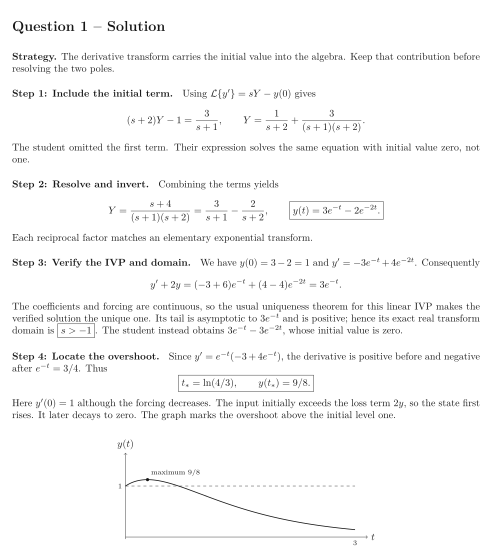
Step 4: Locate the overshoot. Since $y'=e^{-t}(-3+4e^{-t})$, the derivative is positive before and negative after $e^{-t}=3/4$. Thus $$\boxed{t_* =\ln(4/3),\qquad y(t_*)=9/8.}$$ Here $y'(0)=1$ although the forcing decreases. The input initially exceeds the loss term $2y$, so the state first rises. It later decays to zero. The graph marks the overshoot above the initial level one.