Question 5
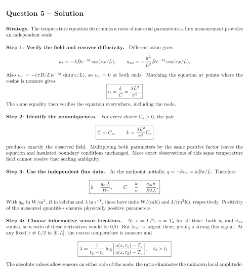
A homogeneous rod with insulated ends is observed to have temperature The unknown constant conductivity and volumetric heat capacity satisfy and . Assume are known.
Tasks
Verify the boundary conditions and infer the diffusivity from the observed field.
Prove that temperature observations of this field alone do not identify and separately. Describe the full family of positive parameter pairs.
An independent measurement gives rightward heat flux per area at . Recover and uniquely and check their units.
Explain why the midpoint is useful for this flux measurement but useless for measuring the temperature decay. Identify which temperature sensor locations can recover from two distinct measurement times.
Show solutionHide solution
Question 5 – Solution
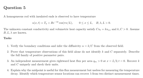
Strategy. The temperature equation determines a ratio of material parameters; a flux measurement provides an independent scale.
Step 1: Verify the field and recover diffusivity. Differentiation gives Also , so at both ends. Matching the equation at points where the cosine is nonzero gives The same equality then verifies the equation everywhere, including the node.
Step 2: Identify the nonuniqueness. For every choice , the pair produces exactly the observed field. Multiplying both parameters by the same positive factor leaves the equation and insulated boundary conditions unchanged. More exact observations of this same temperature field cannot resolve that scaling ambiguity.
Step 3: Use the independent flux data. At the midpoint initially, . Therefore With in , in kelvins and in , these have units and , respectively. Positivity of the measured quantities ensures physically positive parameters.
Step 4: Choose informative sensor locations. At , for all time: both and vanish, so a ratio of these derivatives would be . But is largest there, giving a strong flux signal. At any fixed in , the excess temperature is nonzero and The absolute values allow sensors on either side of the node; the ratio eliminates the unknown local amplitude.