Question 2
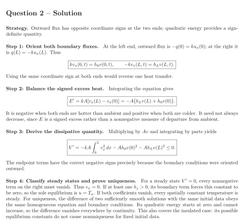
A homogeneous rod of length and constant area obeys , with and insulated sides. Both ends exchange heat with an ambient temperature . The outward heat flux per area equals at end , where . Set and use the signed flux toward increasing .
Tasks
Derive the two boundary conditions, explaining the different signs at the left and right ends.
Derive the rate of change of the total excess heat . Must this signed quantity always decrease?
Derive a dissipation identity for .
Use the identity to classify every steady state, including , and prove uniqueness for a prescribed initial temperature profile.
Show solutionHide solution
Question 2 – Solution
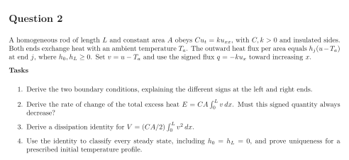
Strategy. Outward flux has opposite coordinate signs at the two ends; quadratic energy provides a sign-definite quantity.
Step 1: Orient both boundary fluxes. At the left end, outward flux is ; at the right it is . Thus Using the same coordinate sign at both ends would reverse one heat transfer.
Step 2: Balance the signed excess heat. Integrating the equation gives It is negative when both ends are hotter than ambient and positive when both are colder. It need not always decrease, since is a signed excess rather than a nonnegative measure of departure from ambient.
Step 3: Derive the dissipative quantity. Multiplying by and integrating by parts yields The endpoint terms have the correct negative signs precisely because the boundary conditions were oriented outward.
Step 4: Classify steady states and prove uniqueness. For a steady state , every nonnegative term on the right must vanish. Thus . If at least one , its boundary term forces this constant to be zero, so the sole equilibrium is . If both coefficients vanish, every spatially constant temperature is steady. For uniqueness, the difference of two sufficiently smooth solutions with the same initial data obeys the same homogeneous equation and boundary conditions. Its quadratic energy starts at zero and cannot increase, so the difference vanishes everywhere by continuity. This also covers the insulated case: its possible equilibrium constants do not cause nonuniqueness for fixed initial data.