Question 1
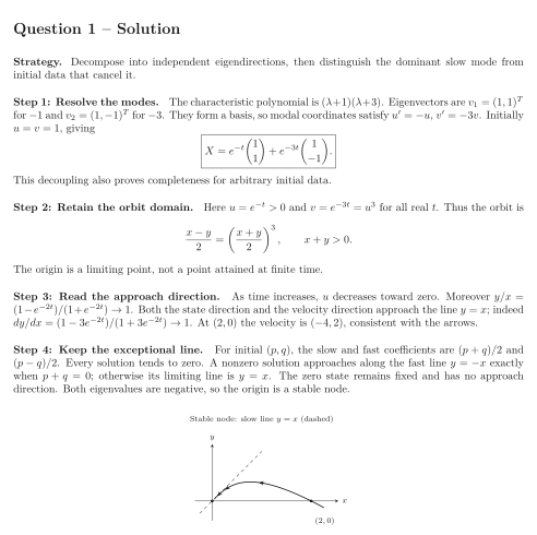
Let solve For geometric interpretation use modal coordinates and . A stable node means that all nearby states tend to the origin forward in time, with two real negative eigenvalues.
Tasks
Find both eigenpairs and solve the IVP. Explain why the two modes give every solution.
Eliminate time for this IVP in the coordinates, retaining the domain. Translate the result to the original phase plane.
Determine the time direction and the limiting tangent line at the origin. Find .
For arbitrary , identify precisely the initial states that approach along the faster eigendirection instead. Classify the origin.
Show solutionHide solution
Question 1 – Solution
Strategy. Decompose into independent eigendirections, then distinguish the dominant slow mode from initial data that cancel it.
Step 1: Resolve the modes. The characteristic polynomial is . Eigenvectors are for and for . They form a basis, so modal coordinates satisfy , . Initially , giving This decoupling also proves completeness for arbitrary initial data.
Step 2: Retain the orbit domain. Here and for all real . Thus the orbit is The origin is a limiting point, not a point attained at finite time.
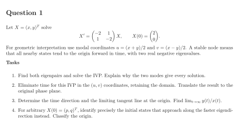
Step 3: Read the approach direction. As time increases, decreases toward zero. Moreover . Both the state direction and the velocity direction approach the line ; indeed . At the velocity is , consistent with the arrows.
Step 4: Keep the exceptional line. For initial , the slow and fast coefficients are and . Every solution tends to zero. A nonzero solution approaches along the fast line exactly when ; otherwise its limiting line is . The zero state remains fixed and has no approach direction. Both eigenvalues are negative, so the origin is a stable node.
See the diagram in the original worksheet below.